My Cribsheet for Dynamical System

The most general (and maybe most important) fact I know about differential equations is that: we generally do not know how to solve them. There are some very simple or very luckily pretty equations that people have systematically solved. For the rest of infinitely many unsolvable equations, one can only analyze them if not devoted to a career of solving them.

1 Ordinary Differential Equation (ODE)

The term "ordinary" is used in contrast with partial differential equations (PDE) which may be with respect to more than one independent variable.

There are several properties that we use to categorize ODEs.

• Order: a $n$$n$-th order ODE only involves the $n$$n$-th and lower order derivatives of $x$$x$.

• Linear: the ODE is linear with respect to the unknown $x$$x$ and its derivatives.

• Homogenous: homogeneous is a prefix used on top of linear ODEs, meaning all terms in the linear ODE are either $x$$x$ or derivatives of $x$$x$.

1.1 First-Order Linear ODE

First-Order Linear Homogeneous ODE

A general first-order linear homogeneous ODE can be written as

The solution is straight-forward. We separate variables and integrate both sides:

First-Order Linear Non-homogeneous ODE

A general first-order linear non-homogeneous ODE can be written as

Its solution is

The first component of the solution is the same as the solution to the homogeneous ODE (the solution when $q(t)=0$$q(t)=0$), which is called the homogeneous solution (齐次方程的通解). The second component of the solution is called the particular solution (非齐次方程的特解). The total solution is the sum of the homogenous solution and the particular solution.

1.2 Second-Order Linear ODE with Constant Coefficients

For second-order linear ODEs, we generally do not have solutions if the coefficients are functions of $t$$t$ (like $p(t),q(t)$$p(t), q(t)$ in first-order linear ODEs we have tackled). We thus tackle the second-order linear ODEs with constant coefficient:

• Second-Order Linear Homogeneous ODE with Constant Coefficients

  If $f(t)=0$$f(t)=0$, the ODE is homogeneous:

  $$\frac{d^{2}x}{d{t}^2}+p\frac{dx}{dt}+qx=0$$

  We write down the associated characteristic equation

  $$r^2+pr+q=0$$

  For different cases where the characteristic equation has different roots, we have the following solutions to the ODE:

  Roots of $r^2+pr+q=0$$r^2 + pr + q = 0$	Solution of $x^{″}+p{x}^{\prime }+qx=0$$x'' + px' + qx = 0$
  $r_1,r_2$$r_1,r_2$ real and distinct	$x(t)=C_1{e}^{r_{1}t}+C_2{e}^{r_{2}t}$$x(t) = C_1 e^{r_1t} + C_2 e^{r_2t}$
  $r_1=r_2=r$$r_1=r_2=r$	$x(t)=C_1{e}^{rt}+C_{2}t{e}^{rt}$$x(t) = C_1 e^{rt} + C_2 t e^{rt}$
  $r_1,r_2$$r_1,r_2$ complex: $\alpha \pm \beta i$$\alpha \pm \beta i$	$x(t)=e^{\alpha t}(C_1\cos \beta t+C_2\sin \beta t)$$x(t) = e^{\alpha t} (C_1 \cos \beta t + C_2 \sin\beta t)$

• Second-Order Linear Non-homogeneous ODE with Constant Coefficients

  When $f(t)$$f(t)$ is in some simple form, we know the solution to the non-homogenous ODE. Otherwise, generally no idea.

  1. $f(t)=P_m(t)e^{at}$$f(t) = P_m(t) e^{at}$

     One simple form $f(t)$$f(t)$ can take is $f(t)=P_m(t)e^{at}$$f(t) = P_m(t) e^{at}$ where $P_m(t)$$P_m(t)$ notates a $m$$m$-th order polynomial of $t$$t$.

     The total solution of the non-homogeneous ODE is the sum of the homogeneous solution and the particular solution. The particular solution is

     Whether the coefficient coincides with the roots	Particular solution
     $a\ne r_1$$a \neq r_1$ and $a\ne r_2$$a \neq r_2$	$x_{\text{p}}(t)=Q_m(t)e^{at}$$x_{\text p}(t) = Q_m(t) e^{at}$
     $a=r_1\ne r_2$$a = r_1 \neq r_2$	$x_{\text{p}}(t)=t{Q}_m(t)e^{at}$$x_{\text p}(t) = t Q_m(t) e^{at}$
     $a=r_1=r_2$$a = r_1 = r_2$	$x_{\text{p}}(t)=t^2{Q}_m(t)e^{at}$$x_{\text p}(t) = t^2 Q_m(t) e^{at}$

  2. $f(t)=e^{at}(P_m(t)\cos bt+Q_n(t)\sin bt)$$f(t) = e^{at} (P_m(t) \cos bt + Q_n(t) \sin bt)$

     The particular solution when $f(t)$$f(t)$ takes such a form is

     Whether the coefficient coincides with the roots	Particular solution
     $a+bi\ne r_1$$a+bi \neq r_1$ and $a+bi\ne r_2$$a+bi \neq r_2$	$x_{\text{p}}(t)=e^{at}(A_k(t)\cos bt+B_k(t)\sin bt)$$x_{\text p}(t) = e^{at} (A_k(t) \cos bt + B_k(t) \sin bt)$
     $a+bi=r_1\ne r_2$$a + bi = r_1 \neq r_2$	$x_{\text{p}}(t)=t{e}^{at}(A_k(t)\cos bt+B_k(t)\sin bt)$$x_{\text p}(t) = te^{at} (A_k(t) \cos bt + B_k(t) \sin bt)$

     $P_m(t),Q_n(t),A_k(t),B_k(t)$$P_m(t), Q_n(t), A_k(t), B_k(t)$ all denote polynomials of the corresponding order. The constant $k=max(m,n)$$k = \max (m,n)$.

1.3 First-Order Linear Differential Equation System

A first-order linear differential equation system can be written as

where the unknown $\mathbf{x}(t)$${\bf x} (t)$ is a $n$$n$-dim column vector; $\mathbf{P}$$\bf P$ is a $n\times n$$n\times n$ constant square matrix; $\mathbf{q}(t)$${\bf q}(t)$ is a known $n$$n$-dim column vector function.

• First-Order Homogeneous Linear Differential Equation System

  If $\mathbf{q}(t)=\mathbf{0}$${\bf q}(t)=\bf 0$, the differential equation system is homogeneous:

  $$\frac{d\mathbf{x}}{dt}=\mathbf{P}\mathbf{x}$$

  Its solution is

  $$\begin{array}{c}\mathbf{x}(t)=e^{\mathbf{P}t}\mathbf{c}=\left[\begin{array}{ccc}{e}^{{\lambda }_{1}t}{\mathbf{r}}_1& \cdots & e^{{\lambda }_{n}t}{\mathbf{r}}_n\end{array}\right]\left[\begin{array}{c}{c}_1\\ ⋮\\ c_n\end{array}\right]=\sum _{i=1}^n{c}_i{e}^{{\lambda }_{i}t}{\mathbf{r}}_i\end{array}$$

  where ${\lambda }_i,{\mathbf{r}}_i$$\lambda_i, {\bf r}_i$ are eigenvalues and eigenvectors of matrix $\mathbf{P}$$\bf P$; $\mathbf{c}$$\bf c$ is a constant vector determined by initial conditions.

  If you can pretend everything is scalar for one second, the solution looks the same as the first-order linear ODE that we solved in the very beginning --- thanks to the matrix exponential $e^{\mathbf{P}t}$$e^{{\bf P}t}$ that is an awesome vector analogy to scalar exponential. The official definition of a matrix exponential is given by the power series:

  $$e^{\mathbf{P}t}=\sum _{k=0}^{\mathrm{\infty }}\frac{1}{k!}{\mathbf{P}}^k$$

  You can use this definition to prove that the matrix exponential is indeed the solution to our differential equation. But if you are only using it to solve these differential equations, don't get involved in calculating the power series; just calculate the eigenvalues to write out the solution.

• First-Order Non-homogeneous Linear Differential Equation System

  If $\mathbf{q}(t)\ne \mathbf{0}$${\bf q}(t)\neq \bf 0$, the solution is

  $$\mathbf{x}(t)=e^{\mathbf{P}t}[\mathbf{c}+{\int }_{t_0}^t{e}^{-\mathbf{P}s}\mathbf{q}(s)ds]=e^{\mathbf{P}t}\mathbf{c}+e^{\mathbf{P}t}{\int }_{t_0}^t{e}^{-\mathbf{P}s}\mathbf{q}(s)ds$$

  Again, this looks the same as the first-order linear non-homogeneous ODE.

1.4 Higher-Order Linear ODE with Constant Coefficients

Apologies for dragging in another notation for derivatives: $x^{(n)}=\frac{d^{n}x}{d{t}^n}$$x^{(n)} = \frac{d^n x}{dt^n}$.

A univariate linear ODE of order $n$$n$

is equivalent to the following first-order $n$$n$-dim linear differential equation system

Solve this linear differential equation system. The solution to the original $n$$n$-th order ODE lies in the last element of the column vector.

2 Stability Analysis

When a differential equation does not have analytical solutions, we turn to qualitative tools to analyze certain properties of our interest. An important property we are usually interested in is stability --- stability of the solution under small perturbations.

This line of tools were first studied by Lyapunov.

2.1 Fixed Point

The general notion of stability is defined on the solution to a differential equation. The solution $\mathbf{x}(t)=\varphi (t),t\in [t_0,\mathrm{\infty })$${\bf x}(t) = \phi (t), t\in[t_0,\infty)$ is stable if $\mathrm{\forall }ϵ>0$$\forall \epsilon >0$, there exists $\delta =\delta (ϵ)>0$$\delta=\delta(\epsilon)>0$ such that the solution is close to $\varphi (t)$$\phi(t)$, namely,

so long as the initialization is close $|{\mathbf{x}}_0-\varphi (t_0)|<\delta$$| {\bf x}_0 - \phi(t_0) | < \delta$.

This is quite hard.

More often, we talk about the stability of a fixed point, that is a constant solution. Fixed points of the differential equation ${\mathbf{x}}^{\prime }=\mathbf{f}(\mathbf{x})$${\bf x}' ={\bf f} ({\bf x})$ are the zeros of $\mathbf{f}(\mathbf{x})$${\bf f} ({\bf x})$. Let's say ${\mathbf{x}}_e$${\bf x}_e$ is a zero of $\mathbf{f}(\mathbf{x})$${\bf f} ({\bf x})$, that is $\mathbf{f}({\mathbf{x}}_e)=\mathbf{0}$${\bf f} ({\bf x}_e)={\bf 0}$. Then, the constant function $\mathbf{x}(t)={\mathbf{x}}_e$${\bf x}(t) = {\bf x}_e$ is a valid solution to the differential equation. It is called a fixed point because $\mathbf{x}$$\bf x$ initialized at ${\mathbf{x}}_e$${\bf x}_e$ will stay at ${\mathbf{x}}_e$${\bf x}_e$ thereafter. If $\mathbf{x}$$\bf x$ converged to ${\mathbf{x}}_e$${\bf x}_e$ when initialized at a point very close to ${\mathbf{x}}_e$${\bf x}_e$, the fixed point ${\mathbf{x}}_e$${\bf x}_e$ is a stable fixed point.

Visually, you can also look at the time-course trajectories of a dynamical system and roughly tell a fixed point is a stable fixed point if all trajectories converge to that point. Here is a schematic visualization of 4 of the most common kinds of fixed points stolen from Wikipedia.

2.2 Stability Analysis of Linear Dynamical System

For linear dynamical systems, we often whether talk about the zero fixed point ${\mathbf{x}}_e=\mathbf{0}$${\bf x}_e={\bf 0}$​ is stable or not. Consider the linear dynamical system

It is obvious that ${\mathbf{x}}_e=\mathbf{0}$${\bf x}_e={\bf 0}$ is a fixed point. Is it stable?

We know that the solution to this dynamical system is

If all eigenvalues are negative, we can see the system will always converge to zero $\mathbf{x}(\mathrm{\infty })=\mathbf{0}$${\bf x}(\infty)={\bf 0}$. This is indeed the condition for the zero fixed point to be stable. More rigorously, we take complex eigenvalues into account. The zero fixed point ${\mathbf{x}}_e=\mathbf{0}$${\bf x}_e={\bf 0}$ is (asymptotically) stable if and only if all eigenvalues of matrix $\mathbf{P}$$\bf P$ have negative real parts $\text{Re}({\lambda }_i)<0$$\text {Re}(\lambda_i)<0$.

The 2D Case

This picture comes up a lot in anything that relates to dynamical systems. But simply looking at it makes me feel uneasy. Both its merit and sin is that it contains a lot of information.

This picture is about judging what type the zero fixed point is by looking at the determinant and trace of matrix $\mathbf{P}$${\bf P}$ (or matrix $A$$A$ in their notation) in a 2D dynamical system.

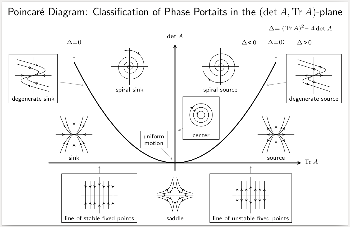
The underlying principle is the same: the zero fixed point is stable if and only if all eigenvalues have negative real parts. For 2D systems, this can be done by looking at the determinant and trace, because the determinant equals the product of all eigenvalues and the trace equals the sum of all eigenvalues. For 2D systems, we have

Equivalently, we have ${\lambda }_1,{\lambda }_2$$\lambda_1, \lambda_2$ are the solution to the quadratic equation ${\lambda }^2-\text{Tr}(\mathbf{P})\lambda +\text{det}(\mathbf{P})=0$$\lambda^2 - \text {Tr} ({\bf P}) \lambda + \text {det} ({\bf P}) = 0$. Hence, $\mathrm{\Delta }=\text{Tr}(\mathbf{P}{)}^2-4\text{det}(\mathbf{P})$$\Delta = \text {Tr}({\bf P})^2 -4 \text {det} ({\bf P})$ can tell us whether the two eigenvalues are real or complex. You can also see that the zero fixed point is stable if the determinant is positive and trace is negative.

2.3 Stability Analysis of Nonlinear Dynamical System

There is not much to add here. For nonlinear dynamical systems, we linearize the dynamics and treat them with linear stability analysis.

"Linearize" means first-order Taylor expansion. This is a legit simplification because stability is a property about how small perturbations influence the system ---- first-order Taylor expansion is usually accurate enough around small perturbations.

Let's be more specific. Consider nonlinear dynamics:

Assume ${\mathbf{x}}_e$${\bf x}_e$ is a fixed point, namely $\mathbf{f}({\mathbf{x}}_e)=\mathbf{0}$${\bf f} ({\bf x}_e)={\bf 0}$. Since we are interested in the dynamics around ${\mathbf{x}}_e$${\bf x}_e$, we linearize the $\mathbf{f}(\mathbf{x})$${\bf f} ({\bf x})$ around ${\mathbf{x}}_e$${\bf x}_e$.

We use $\mathbf{J}$${\bf J}$ to denote the Jacobian matrix, that is the first-order partial derivatives of $\mathbf{f}(\mathbf{x})$${\bf f} ({\bf x})$ evaluated at ${\mathbf{x}}_e$${\bf x}_e$.

Since the dynamics around ${\mathbf{x}}_e$${\bf x}_e$ is well approximated by ${\mathbf{x}}^{\prime }=\mathbf{f}(\mathbf{x})\approx \mathbf{J}(\mathbf{x}-{\mathbf{x}}_e)$${\bf x}' ={\bf f} ({\bf x}) \approx {\bf J} ({\bf x} - {\bf x}_e)$, the question of whether ${\mathbf{x}}_e$${\bf x}_e$ is stable in the nonlinear dynamical system ${\mathbf{x}}^{\prime }=\mathbf{f}(\mathbf{x})$${\bf x}' ={\bf f} ({\bf x})$ can be answered by whether $\mathbf{0}$$\bf 0$ is stable in the linear dynamical system ${\mathbf{x}}^{\prime }=\mathbf{J}\mathbf{x}$${\bf x}' = {\bf J} {\bf x}$.

3 From A Signal Processing Perspective

Signal Processing provides a very nice perspective on dynamical systems, especially linear dynamical systems.

Green Function

Green function is the impulse response of a nonhomogeneous linear differential operator with specified initial or boundary conditions. If knowing the Green function, the convolution between the Green function and the nonhomogeneous term gives us a particular solution to the nonhomogenouse ODE.

Proof I

Green Function is usually a late chapter in a differential equation textbook. But the impulse response is often the first chapter in a signal and system textbook. This is probably because its proof looks quite simple there.

In the signal and system context, the system is not necessarily defined by differential equations. It can be any linear time-invariant (LTI) systems.

Let us assume the impulse response of a LTI system is $g(t)$$g(t)$, that is

Since the system is time-invariant, we can shift the time by $t^{\prime }$$t'$

Since the system is linear, we can scale both sides by $f(t^{\prime })$$f(t')$

We then integrate both sides and finishes the proof

The lefthand side is $f(t)$$f(t)$ by the property of the delta function. The righthand side is a convolution between $f(t)$$f(t)$ and $g(t)$$g(t)$.

Proof II

Green function is also the inverse Laplace transform of the inverse of the system's frequency response. Say we have a linear differential operator $\text{L}$$\text L$. We know that $\text{L}$$\text L$ acting on the Green function $G(t)$$G(t)$ gives us the delta function,

We can do Laplace transform on both sides and look at the equation in the frequency domain:

Here $H(s)$$H(s)$ is called the frequency response of the dynamical system. It is a polynomial in linear ODEs with constant coefficients.

Now we are to find the function that gives us $x(t)$$x(t)$ when being acted on by the linear operator $\text{L}$$\text L$,

We do Laplace transform on both sides and get

We can solve the Laplace transform of $x(t)$$x(t)$ by division and Laplace transform back to obtain the solution

Through the Laplace transform procedure, we see that the frequency domain perspective is very useful for solving ODEs because invert a differential operator in the frequency domain is just division.

Solving First-Order Linear ODE with Green Function

Consider a first-order linear non-homogeneous ODE:

Definitions

• Homogeneous solution: solution to $\dot{x}+px=0$$\dot x + px = 0$, which is $x_{\text{h}}(t)=c{e}^{-pt}$$x_{\text h}(t)=ce^{-pt}$.

  The homogeneous solution is unique when an initial condition is given.

• Particular solution: solutions to $\dot{x}+px=q(t)$$\dot x + px = q(t)$ that hold for any initial condition, one of which is $x_{\text{p}}={\int }_{t_0}^{t}q(t^{\prime })e^{-p(t-t^{\prime })}d{t}^{\prime }$$x_{\text p} = \int_{t_0}^t q(t') e^{-p(t-t')}dt'$.

  The particular solution is not unique (providing initial conditions won't help, $x_{\text{p}}$$x_{\text p}$ just doesn't concern initial conditions).

• Green function: solution to $\dot{x}+px=\delta (t)$$\dot x + px = \delta(t)$ with a specified initial condition, usually $x(0)=0$$x(0)=0$. The Green function with zero initial condition is $g(t)=e^{-pt}\mathrm{\Theta }(t)$$g(t)=e^{-pt} \Theta (t)$.

  The Green function is unique subject to the initial condition. Note that the Green function often resembles the homogeneous solution, because they should behave the same except at $t=0$$t=0$.

Solutions

• Sum of Homogeneous and Particular Solution

  The solution of a linear non-homogeneous ODE is the sum of its homogeneous and particular solution. To make the solution unique, suppose we know the initial condition $x(0)=x_0$$x(0)=x_0$​​. Then the solution is

  $$x(t)=x_{\text{h}}(t)+x_{\text{p}}(t)=x_0{e}^{-pt}+{\int }_0^{t}q(t^{\prime })e^{-p(t-t^{\prime })}d{t}^{\prime }$$

• Convolution of Green Function and Non-homogeneous Input

  Convolution of the Green function and non-homogeneous input gives us a particular solution to the non-homogeneouse ODE.

  $$x_{\text{p}}(t)=q(t)\ast g(t)={\int }_0^{\mathrm{\infty }}q(t^{\prime })e^{-p(t-t^{\prime })}\mathrm{\Theta }(t-t^{\prime })d{t}^{\prime }={\int }_0^{t}q(t^{\prime })e^{-p(t-t^{\prime })}d{t}^{\prime }$$

  For zero initial condition $x(0)=0$$x(0)=0$, this is the complete solution since the homogeneous solution is zero. For nonzero initial conditions, this is a particular solution.

Remark: Since I am a little paranoid about writing the complete solution as a convolution, I find that this is possible but not pretty. The complete solution is